Introduction

Offshore investing is a powerful strategy to preserve and grow your wealth. It allows Performance evaluation is one of those topics that may be easy to understand conceptually, but your understanding can begin to fall apart once you get into the detail.

Fortunately, there are great frameworks for thinking about this ‘problem’, and great tools for helping with the exercise. In this article, we will tackle the problem from the perspective of uncertainty, which will be useful for everyone in the value chain, all the way from investors to the asset managers who ultimately make the security selection and asset allocation decisions.

The topic is complex so we will begin by providing an introduction on some of the fundamental concepts that need to be understood in tackling this complexity.

Why evaluate performance?

The purpose of performance evaluation is to understand how something measures up against expectations or goals and objectives. An investor, adviser, or DFM may want to understand how an appointed asset manager has performed relative to its benchmark. Alternatively, an investor may want to understand how an adviser/DFM has performed relative to other advisers/DFMs.

There are many reasons for performance evaluation but if we focus on the objective of understanding performance, we realise that the purpose is ultimately to get actionable information. That information could result in the hiring or firing of an asset manager. To get to that decision, however, we need to understand investments intimately, so that we recognise the limitations of the exercise, and hence the limitations on decisions we take. This requires an understanding of the uncertainty inherent in performance evaluation.

Framework

There are many different frameworks for tackling performance evaluation, but we will focus on an easy to understand and well recognised framework, that is taught by the CFA Institute in their Certificate in Investment Performance Measurement. Essentially, performance evaluation consists of three main components, namely: performance measurement, performance attribution and performance appraisal. Let us look at these in a little more detail.

Performance measurement is the starting point and is measures the performance realised. This may appear to be a relatively

simple exercise, but it comes with lots of complexity, so let us unpack the concept a little further by asking a couple of related

questions, such as:

• Are we measuring returns, risk, or something else, such as costs?

• Are we measuring a client account, a fund, or a composite of funds or accounts?

• Are we measuring returns gross or net of fees and costs?

• Over what period are we measuring? Or are we interested in multiple periods?

• Are we measuring performance against a benchmark, an objective or peers?

• What return measure are we using, for example, time-weighted or money-weighted, and what formula is required?

These are just some of the important questions we need to understand before embarking on measuring performance.

Performance attribution is the next step and looks at how the performance observed was derived. Again, there are many ways to ‘slice and dice’ this analysis, but that does not mean that they are all equally valid. It is important to understand the manager’s (or adviser’s) investment philosophy and process so that the appropriate analysis can be performed. Not doing so may lead to drawing conclusions from faulty analysis. A quick example will help to explain this. Let us assume that an asset manager has been appointed to manage a sovereign bond mandate. It would be a grave mistake to measure that asset manager’s performance relative to a credit bond benchmark or credit bond peers.

Performance appraisal is the final step in the process but is the most important. Unfortunately, most performance evaluation exercises stop before this step is adequately completed and therefore nothing results from the previous two steps. This step is concerned with the decision-making element of performance evaluation, by asking “so what?” What can be deduced or inferred from the performance measurement and attribution and what action, if any, should be taken. If performance was bad (or good), and the attribution points to sources of the returns which would not have been expected, should a manager be fired (or hired)? There are many possible implications for the results of the appraisal, and understanding the analysis is critical if you are to make good decisions from the results.

Past performance used as the only dimension to perform appraisal

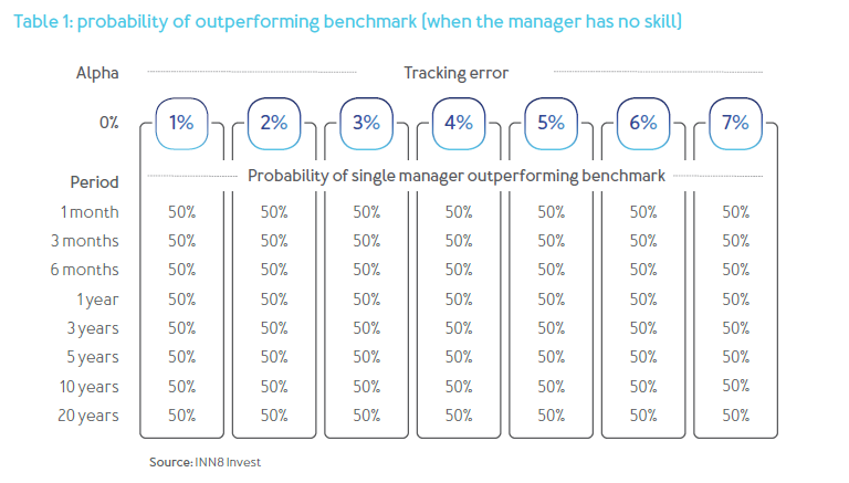
If your analysis was simply to consider whether a manager has outperformed an appropriate benchmark or not, you should expect half of all managers with ‘no skill’ to outperform over any time period (no matter how long). So looking at past performance is as good as flipping a coin for decision making - that is, it is worthless. Table 1 illustrates this point.

That is why using past performance as the only input in deciding whether an asset manager is skillful or not, is a waste of time - especially if the analysis is done using flawed methodologies (which it very often is).

While we could fill a textbook with all the information required to unpack this topic completely, we will instead try to cover the high-level summary.

More dimensions required to appraise manager skill – time period and tracking error

If the analysis were to focus on the managers achieving a minimum level of alpha (say 1%, gross), then the probability of managers with no skill achieving this will fall as the time period of the analysis increases. The table that follows demonstrates these probabilities along two dimensions under idealised assumptions. The first dimension is the time period used for the analysis, which is observed by looking at the rows along the leftmost column. The second dimension is tracking error (or active risk), observed by looking at the columns along the top row.

There is a lot of useful information in this table, so let us examine some of it:

• Firstly, the probabilities of outperforming the benchmark by 1% drop as the period increases, for any given level of tracking error. This is analogous to how casinos operate. With the odds slightly in their favour, the probability of them making money increases as the number of independent bets increases. This can be explained using another classic example, namely flipping a coin. If you had an unbiased coin (equally likely to land on heads or tails), and you flipped it many times, the chance of you getting a value far above or below the 50% mark (for heads or tails), would drop with the number of flips. For example, the chance of you flipping 60% heads (or more) in ten flips of the coin i.e. 6 heads or more, would be around 13% (not very likely, but certainly not rare). If, however, you flipped the coin 50 times, the chance of you flipping 60% heads (or more) would drop to 6% (less than half the previous probability). The probability would decrease further the more you kept flipping.

• Secondly, the probabilities increase with tracking error for any given period. Another example can be used to help us understand this - insurance is a great example of uncertainty. Imagine you had two different insurers, offering two different kinds of cover. The one offers cover on regular cars with an average cost of R100 000. The other offers cover on high performance cars which cost on average R1 million. The probability of a car crash is exactly the same in both cases (but not true in reality), and the insurer collects enough in premiums to cover the cost of the risk (also not true in practice, as insurers need to cover a plethora of additional costs). Let us now assume that both insurers have exactly the same amount in rands of cars under insurance — say R100 million, which implies 1 000 cars for the first insurer, and 100 cars for the second insurer). If both decided to hold just R1 million additional capital to ensure that they could meet all claims, would they have the same probability of failure? The answer is no, the second insurer would only be able to suffer one additional loss more than expected before running out of capital, whereas the first insurer could suffer an additional 10 losses - a much less likely event.

• This may however be counter-intuitive for some who have read that managers will hug the benchmark so that they are not caught out for having no skill (through underperformance). While this is correct as the probability of underperforming by any amount greater than 0% (ignore the special case of 0%) will similarly increase with the holding period, there is still a reason for managers to take more risk, which is that the chance of outperforming also increases, and represents a free option on clients’ assets.

• Increasing the hurdle (alpha) from 1% to 2%, will drop all of the probabilities, but more so for the bottom left half of the table (triangle), as per Table 3 over the page.

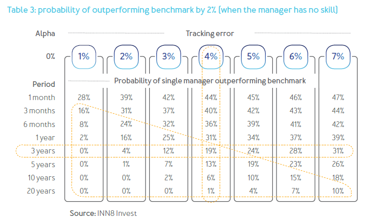
So how could you legitimately use past performance in a performance evaluation exercise, and what does the analysis in Table 3 tell us about the pitfalls of doing so?

If we were to change the hurdle to 2% and consider a manager with a tracking error of 4%, we can calculate that the probability of outperformance drops to 19% for a period of three years, from 40% for three months. The implication is that a manager with no skill is half as likely to outperform that hurdle if you consider the performance over three years instead of three months, which in turn implies that you are half as likely to erroneously assume that the manager has skill - although there is still a one in five chance of you being wrong.

What if you were to increase the tracking error to 6% (a 50% increase)? What time frame would now be appropriate to get back to the same probability? Again, we can calculate that the time period would now need to be increased to seven years (a 133% increase).

So, you should begin appreciating that time and tracking error are two important dimensions in performance evaluation.

Probabilities and expectations – another dimension

Just like statistics are not intuitive, probabilities are sometimes worse. How often have you heard (or said) that weather forecasters have no idea what they are doing, because they said there was only a 30% chance of rain, and it rained (or similarly, not equivalently, there was a 70% chance of rain, and it did not rain). People often assume that low probability events do not occur but are very often happy to gamble on low probability events, such as the lottery.

To properly assess the skill of a weather forecaster, you would need to compare their predictions to reality over many observations, not just a few, and certainly not just one. For example, if you observed that there were 100 times that the forecaster said that the chance of rain was only 30%, you should expect it to rain 30 times (plus or minus some reasonable

error, which you can calculate if you want to make some further assumptions about how confident you want to be in the result). Now expecting it to rain 30 times out of a hundred is very different from not expecting it to rain.

How does this translate into performance evaluation? Well, if you now consider the 19% probability referred to above (Table 3), it means that 19 out of 100 times you would still be wrong, even though you were careful to extend the performance evaluation period from three months to three years for a manager with a tracking error of 4%. So, you would be assuming that the manager was skillful because they had outperformed the benchmark by 1% over three years, and this was unlikely to occur by chance.

This is equally important when evaluating manager performance in the context of the investment decisions they make. For example, if a manager had to invest in a particular company based on a low probability event that would make the company very profitable (say a blockbuster drug), and the event does not occur and hence the investment turns out to have been a poor investment, would this represent a bad decision? You actually should not be making this assessment based on a single investment, because the probability of the event is critical.

If the event was expected to have a probability of 1% (this could still make sense from an investment thesis point of view if the expected return was sufficiently high), you would need to assess many of these low probability events together. In this case, 100 such events would not be enough to have much confidence in your assessment because 1% of 100 is only 1, making a zero events outcome quite likely.

So prior probabilities and expectations are another important dimension in performance evaluation. There are many other important considerations when doing performance evaluation, required to ensure that the analysis is meaningful and the conclusions are robust. Unfortunately, we have only scratched the surface on this very important topic.

Conclusion

You may come away from reading this with a sense that we have not provided you with solutions, but rather only highlighted some of the pitfalls. This is intentional and important because we often see people seeking refuge in numbers (calculated very precisely), believing that they hold the answers. This article was meant to give you a sense of the uncertainty that remains, even when doing the analysis robustly, and why decision making in the context of uncertainty is important.

We should never throw the baby out with the bath water. Understanding the uncertainty allows us to better appreciate what confidence we should have in the decisions we take, and what outcomes we should expect when observed over multipleobservations.